Stereo Matching

Objectives & Main Features

The objectives of the project were to explore the performance difference of various stereo matching methods including Sum of Absolute Differences, Sum of Squared Differences, Normalized Cross Correlation and Semi-global matching (SGM), as well as the choosing of parameters such as kernel size. Intel Realsense D455 RGB-D camera was used to collect the stereo image pairs. The Intel Realsense RGB-D camera could emit infrared ray to assist the depth estimation by adding extra features to some surface without feature such as white walls. Therefore, whether the infrared ray could help generate better depth map will be tested and discussed.

Steps & Implementation

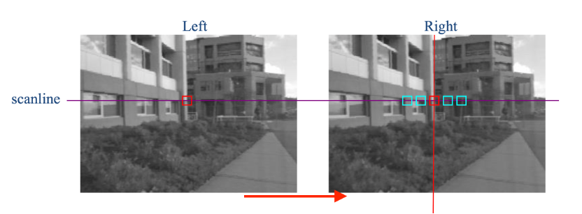
In general, the matching procedure could be executed as shown in the flowchart in Figure 2. The idea was to find the same point in the real world in both left and right image. Usually, as shown in Figure 1, a kernel (a square area) was firstly chosen in one image, for example, the left image. Then, starting from the same position as the kernel in the left image, a horizontally sliding kernel was created in the right image and the cost between the kernel in the left image and the sliding kernel in the right image was calculated. The cost function could be modified. The kernel position with the least cost in the sliding range, which could also be modified, in the right image was considered as a match to the left kernel. The pixel distance between the position of the left kernel and the one in the right image was the disparity. As the closer the object is, the larger the disparity is. The sliding range decided the closest distance that the depth map could be generated.

Three different cost functions, which were SAD, SSD and NCC, were implemented and the performance for each cost function will be discussed in the next section.

Sum of Absolute Differences (SAD)

$$\sum_{\left(i,j\right)\in W}\left|I_1\left(i,j\right)-I_2\left(x+i,y+j\right)\right|$$

Sum of Squared Differences (SSD)

$$\sum_{\left(i,j\right)\in W}\left(I_1\left(i,j\right)-I_2\left(x+i,y+j\right)\right)^2$$

Normalized Cross Correlation (NCC)

$$\frac{\sum_{\left(i,j\right)\in W}{I_1\left(i,j\right)\bullet I_2\left(x+i,y+j\right)}}{\sqrt[2]{\sum_{\left(i,j\right)\in W}{{I^2}_1\left(i,j\right)}\bullet\sum_{\left(i,j\right)\in W}{{I^2}_2\left(x+i,y+j\right)}}}$$

Semi-global Matching (SGM) - Census Transform & Hamming distance

The previous methods used the sum of the cost for each pixel in the kernel between the left and right image to find the best match. In another words, the sum of the pixel value difference was used as the feature that the matching process referred to.

For the scene with little illumination change and with relatively high number of features, SAD, SSD and NCC may find pretty good matches. However, if the illumination condition was different in two images, the matching will be greatly influenced because the mean pixel value will be different even if for the same part of the image.

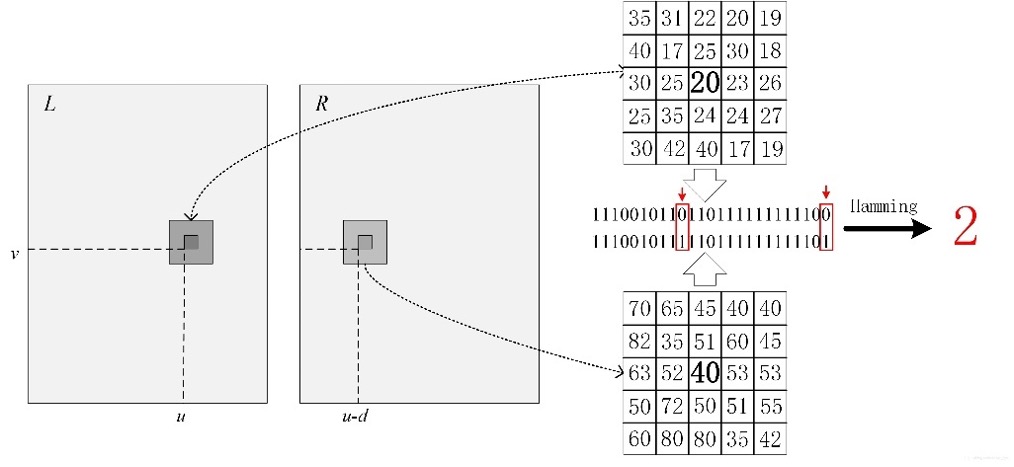
Census transform used the pixel difference between the certain pixel with the adjacent pixels as the feature for matching. Therefore, it could be considered the pattern of changing for each pixel was used. As shown in Figure 3, the census transform was to compare the value of the center pixel and the pixels around it. If the adjacent pixel was larger, encode ‘1’ while the center pixel was larger, encode ‘0’. Then, the binary code series of the kernel in left and right images did ‘XOR’ operation, the output was called Hamming distance, which could be considered as cost. The best match should have the smallest Hamming distance.

Results

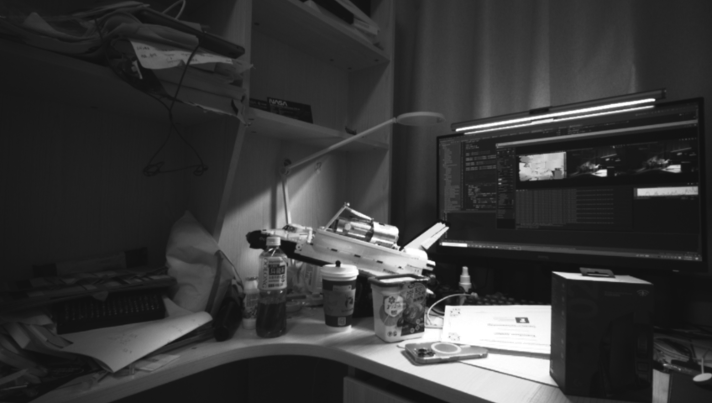
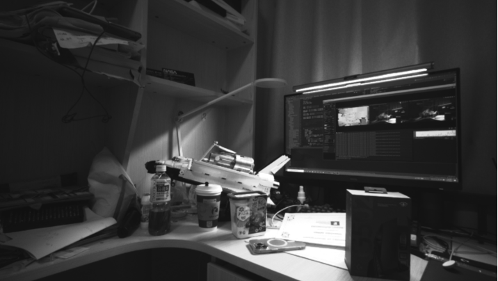
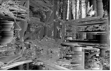
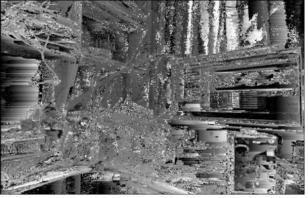
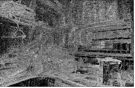
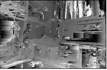
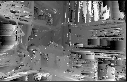
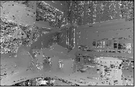
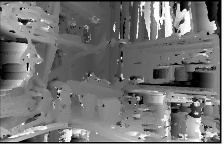
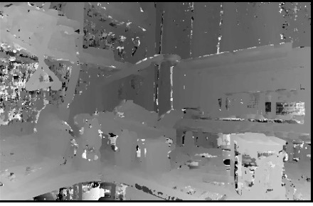
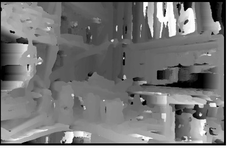
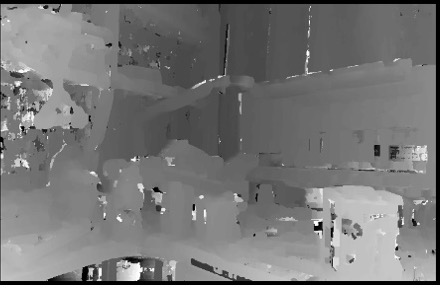
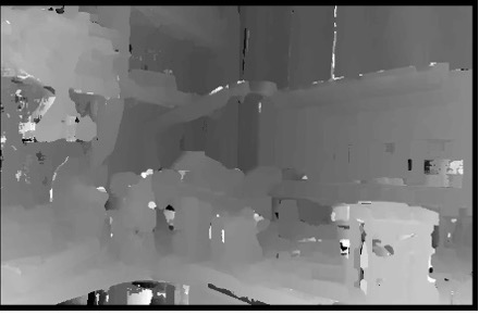
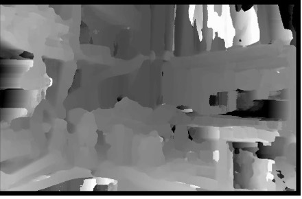
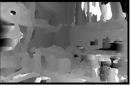
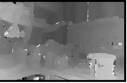
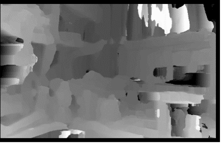
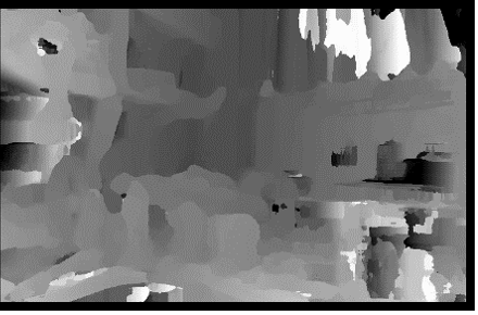
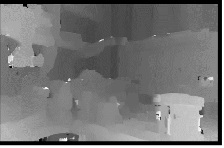
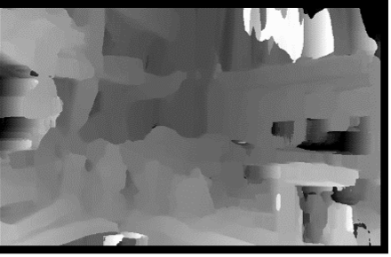
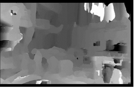
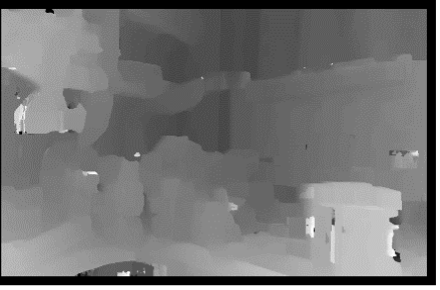
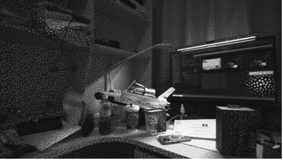
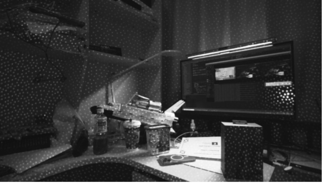
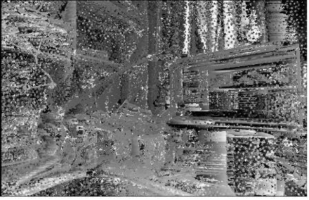
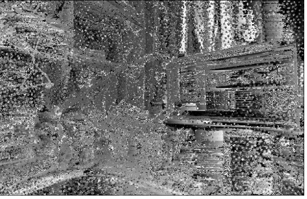
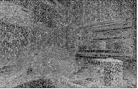
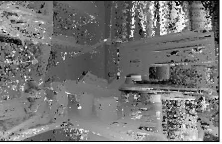
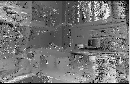
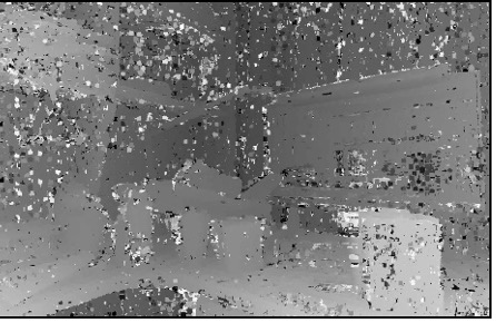
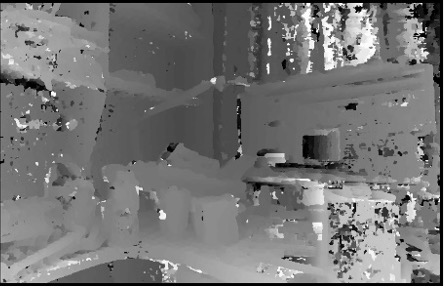
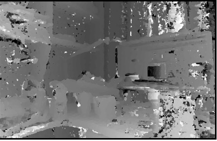
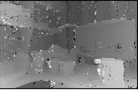
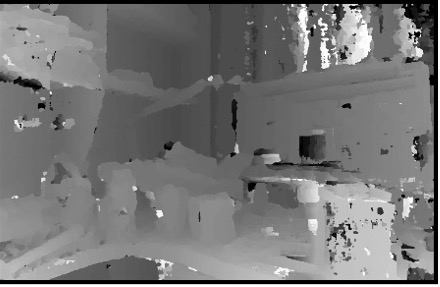
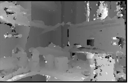
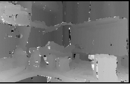
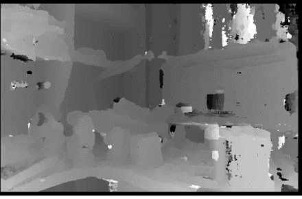
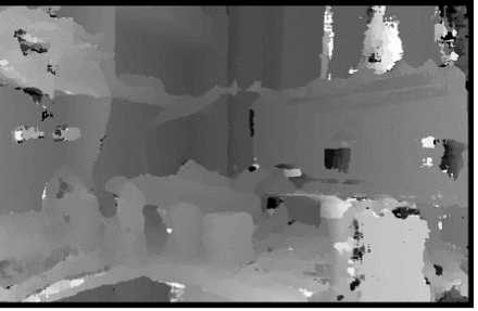
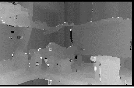
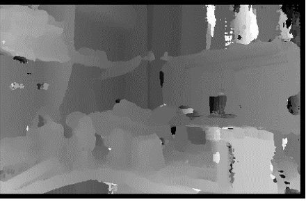
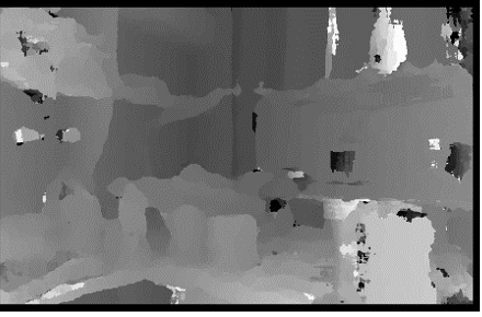
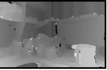
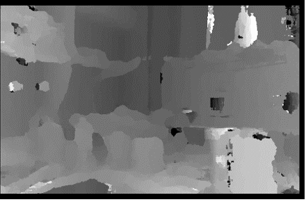
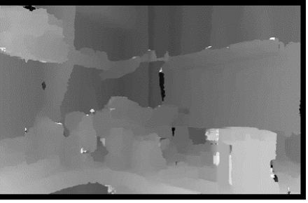
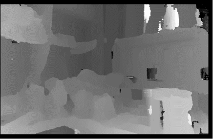
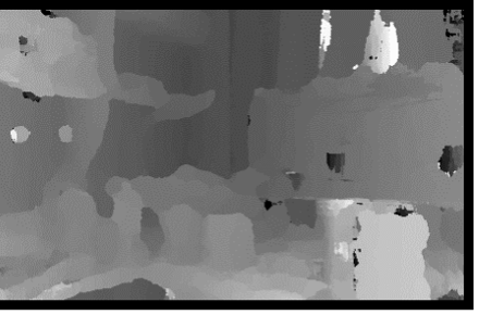
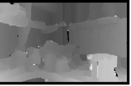
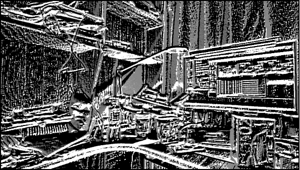
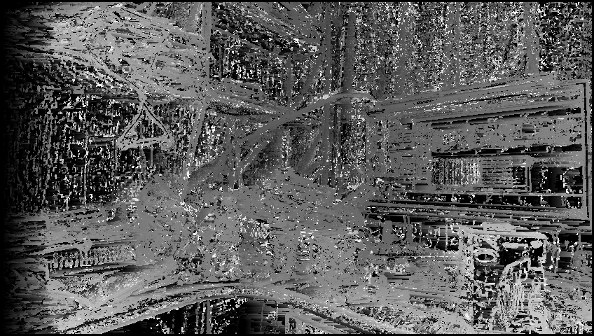
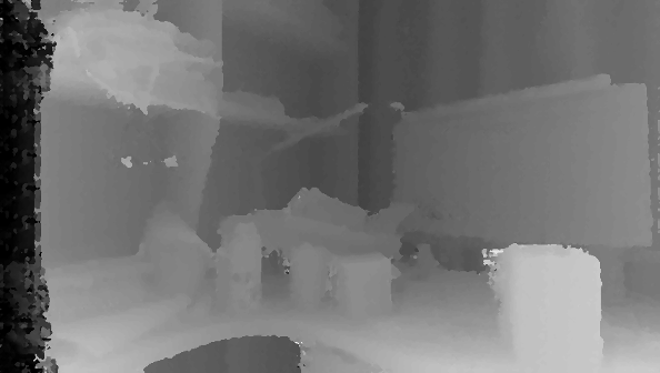
Three aforementioned cost functions were tested with different size of kernels. Moreover, as Intel Realsense RGB-D camera, which could actively emit infrared ray with a fixed pattern to assist on-chip stereo matching on the camera, was used to collect stereo images, the stereo matching performance with or without the assistance of infrared ray was tested and compared as well. The collected images were self-rectified before output from the camera. Therefore, the images were used directly for stereo matching. The resolutions of the images for matching were 848*480. Figure 4 and Figure 5 were the image captured without infrared ray while Figure 6 and Figure 7 were the image captured with infrared ray on. The largest disparity was set to 100 for completed depth calculation.

Without Infrared Laser:

	SAD	SSD	NCC
3
7
11
15
19
23
27
31

With Infrared Laser:

As the figures in Table 1 and 2 shown, for both laser-assisted and normal images, the depth map generated by kernels with smaller sizes were noisier and with a greater number of pixels that failed to be matched. However, it could be observed that although the depth maps generated with large kernels were smoother, they lost some of the details of the objects in the image such as the sharpness of their shapes. The reason for this phenomenon might be that small kernels will have large changes in values when sliding, therefore, it was relatively easy to match to a random area that was similar to the correct target. On the contrary, large kernels were relatively consistent in values, so that large kernels may not reflect small details but will be more likely to be smooth. Among three different cost functions, it was apparent that the normalized cross correlation (NCC) gave matching results with less noise and more valid matching pixels than the other two methods did. By using NCC, the improvement was mainly in the area that was with little strong features. In the images generated by the non-laser image pairs, the depth maps generated by NCC cost function were more obviously better than the other two cost functions.

Compared the results obtained by the images with infrared lasers with the ones without the assistance of the infrared lasers, it was obvious that the laser-assisted results were much more detailed, for example, sharp edges on objects, and with less failed pixels especially in the area that was lack of features. In the three tested methods, only NCC could give reasonable matching results without the assistance of infrared ray.

Table 3. The duration for calculating the matching (unit: seconds)

	SAD	SSD	NCC
3
7
11
15
19
23
27
31

	3	7	11	15	19	23	27	31
SAD	101.576	101.225	101.731	103.691	104.877	107.071	110.637	112.446
SSD	138.111	141.071	144.934	151.417	160.569	167.141	189.495	205.365
NCC	255.229	273.032	259.001	271.406	278.993	299.047	324.951	336.753

As for the time cost to calculate the matching, SAD cost function took the shortest time to calculate the matching and NCC was the most time-consuming one. Moreover, the larger the kernel was, the slower the calculation was. This trend was applied to all three methods because larger kernels simply led to more computation for each round of cost calculation.

These three methods all cost more than one minute to generate only one depth map, which was too slow for some application like robotic vision that needed very high real-time performance. One possible solution was to used FPGA to calculate the depth because the calculation in stereo matching can be executed in parallel. It was speculated that Intel Realsnese RGB-D camera used FPGA inside the camera to do the stereo matching.

It could be observed that the depth was changing smoothly on surfaces and was sharp on the edges. The scene was naturally presented, and objects could be clearly recognized in the depth map.

Conclusion

In conclusion, the window-based stereo matching performance with three different cost functions, which were SAD, SSD and NCC, was discussed. It was found that NCC had the best matching performance while it took the longest time to compute. Moreover, the projection of infrared ray was proved to be effective to generate depth maps with higher quality because it could add extra features to the field of view so that the matching algorithms could find the correct match with less effort, especially for the area with little strong features. Additionally, the matching algorithm needed to be implemented on specially designed FPGA for real-time operation.